On Quantum Teleportation
Continuing a little bit the quantum subjects. I was re-reading quantum teleportation and I was asking to myself. Why do they use always the $T_2$ triplet? (In theoretical minimum notation). I was thinking in that concept and I realized it’s one of the EPR pairs or state $|\Phi^+\rangle$ according to wikipedia. By the way, the book Quantum Computation and Quantum Information calls it simply the EPR pair.
I decided then that I would give a go to at least another bell state as well a properly trying everything in a quantum computer.
Anyway, firstly, there exists a theorem in quantum mechanics which states that you cannot simply make an exact copy of an unknown quantum state. This is known as the no-cloning theorem, there is a proof of the statement as well in the article.
Theory (1st Part)
Let’s start with some theory. Let’s say we have a state $|\psi\rangle$ which might contain any value. $$ \begin{equation} |\psi\rangle = \alpha|0\rangle + \beta|1\rangle \end{equation} $$
Our objective is to be able to pass that state to another qubit.
$$ \begin{align} |e \rangle = \frac{1}{\sqrt{2}} (|00\rangle + |11\rangle) \end{align} $$
This entangled qubits can be separated by a big distance. And hence the teleportation naming, once you have the state, you can know the other state due to the entanglement. On a different note, $|e \rangle=|\Phi^+\rangle$, in section Theory (2nd Part) we’ll try to use another EPR pair.
Now, let’s do the tensor product of the two precedent variables.
$$ \begin{align*} \begin{aligned} |\psi\rangle \otimes |e\rangle &= \frac{1}{\sqrt{2}} (\alpha |0\rangle \otimes (|00\rangle + |11\rangle) + \beta |1\rangle \otimes (|00\rangle + |11\rangle))\\ &= \frac{1}{\sqrt{2}} (\alpha|000\rangle + \alpha|011\rangle + \beta|100\rangle + \beta|111\rangle) \end{aligned} \end{align*} $$
That’s our 3 states qubit $|q_0 q_1 q_2\rangle$. We want to pass the value from $q_0$ to $q_2$. Let’s now perform the operations to translate the information.
$$ \begin{align*} \begin{aligned} &(H \otimes I \otimes I) (CNOT \otimes I) (|\psi\rangle \otimes |e\rangle)\\ &=(H \otimes I \otimes I) (CNOT \otimes I) \frac{1}{\sqrt{2}} (\alpha|000\rangle + \alpha|011\rangle + \beta|100\rangle + \beta|111\rangle) \\ &= (H \otimes I \otimes I) \frac{1}{\sqrt{2}} (\alpha|000\rangle + \alpha|011\rangle + \beta|110\rangle + \beta|101\rangle) \\ &= \frac{1}{2} (\alpha(|000\rangle + |011\rangle + |100\rangle + |111\rangle) + \beta(|010\rangle + |001\rangle - |110\rangle - |101\rangle)) \\ \end{aligned} \end{align*} $$
$$ \begin{align*} \begin{aligned} = \frac{1}{2}( & \phantom{+} |00\rangle (\alpha|0\rangle + \beta|1\rangle) \hphantom{\quad )} \\ & + |01\rangle (\alpha|1\rangle + \beta|0\rangle) \hphantom{\quad )}\\ & + |10\rangle (\alpha|0\rangle - \beta|1\rangle) \hphantom{\quad )}\\ & + |11\rangle (\alpha|1\rangle - \beta|0\rangle) \quad )\\ \end{aligned} \end{align*} $$
We can feel that there is some structure and that we are almost there. As you can see, when we read in the 2 most significant qubits and the value is $|00\rangle$, this means that $q_2$ will have the value $\alpha|0\rangle + \beta|1\rangle$ which is exactly the value of $\psi$. So far so good, let’s see the possible states of $q_2$ given our previous equations and the gates that we need to apply given the information of $|q_0q_1\rangle$.
| $|q_0q_1\rangle$ | $|q_2\rangle$ state | Quantum Gate |
|---|---|---|
| $|00\rangle$ | $\alpha|0\rangle + \beta|1\rangle$ | $I$ |
| $|01\rangle$ | $\alpha|1\rangle + \beta|0\rangle$ | $X$ |
| $|10\rangle$ | $\alpha|0\rangle - \beta|1\rangle$ | $Z$ |
| $|11\rangle$ | $\alpha|1\rangle - \beta|0\rangle$ | $ZX$ |
What this means is that, after measuring the first two qubits, we can recover $|\psi\rangle$ in $q_2$ as desired.
Practice (1st Part)
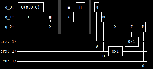
In the practical part, we have to say that as usual, the initial state of our qubits is $|000\rangle$. The first qubit is going to be transformed to the value $|\psi\rangle$ which we are to define. The other two more significant bits are going to be the EPR pair. This we’ll do it with a hadamard gate followed by a controlled X gate. You’ll see the reference in the code with the reference to equation (1) and equation (2).
import matplotlib.pyplot as plt
from qiskit import *
from qiskit.tools.monitor import job_monitor
from qiskit.tools.visualization import plot_bloch_multivector, plot_histogram
from math import pi


qr = QuantumRegister(3, name="q")
crz, crx = ClassicalRegister(1, name="crz"), ClassicalRegister(1, name="crx")
c0 = ClassicalRegister(1, name="c0")
qc = QuantumCircuit(qr, crz, crx, c0)

# this will be the value of equation (1)
# instead of random, we pick, and that's the value that we should
# expect in the end of the algorithm
θ = pi/2
θ = 0
qc.u(θ,0,0,0)

# bell state to obtain equation (2)
qc.h(1)
qc.cx(1, 2)

# algorithm
qc.barrier()
qc.cx(0,1)
qc.h(0)
qc.barrier()
# measurement for teleportation
qc.measure([0, 1],[0, 1])

# implementation of the quantum gate depending on the
# measured state |q_0 q_1> as defined in the table
qc.x(2).c_if(crx, 1)
qc.z(2).c_if(crz, 1)

qc.measure(2,2)

simulator = Aer.get_backend("qasm_simulator")
sim_result = execute(qc, backend=simulator, shots=1024).result()
plot_histogram(result.get_counts())
We can print the quantum circuit with the command qc.draw() which will give us the following drawing of the circuit.

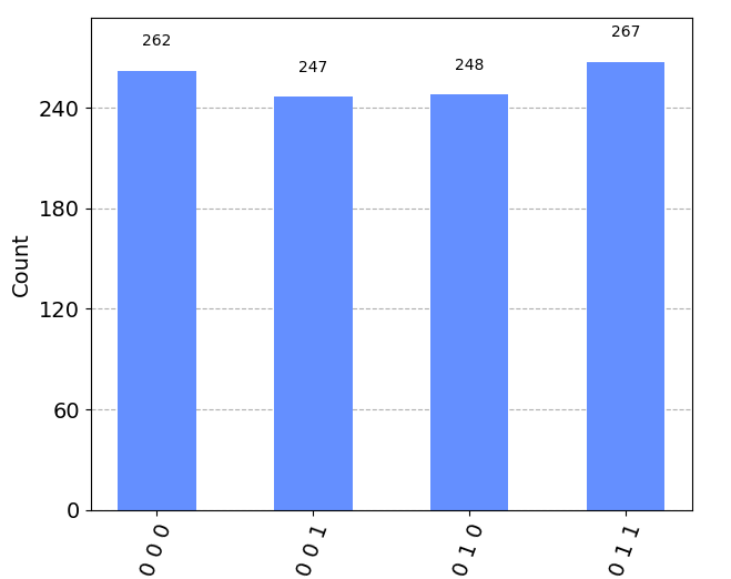
As for the result of plot_histogram(result.get_counts()), here you have 2 images. In the first, $|\phi \rangle=|0\rangle$ (in code θ=0).

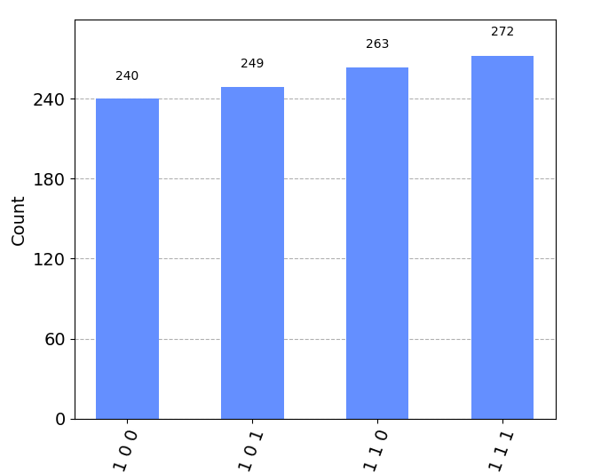
In the second, $|\phi \rangle=|1\rangle$ (in code θ=pi).

Here it’s true that one can use the X gate, however, I wanted to compare with more angles and make it analogous to the previous post on Qubit Rotation.
In the first image, you can see that the most significant value or when $|\phi \rangle=|0\rangle$ is q2=0 and when $|\phi \rangle=|1\rangle$, q2=1. This means that at least for the edge values, everything seems perfect in simulation.
Now, when we want to test in the ibm_perth quantum computer, the code does not work (as for October 2023). We run into the following problem.
Failed - Instruction bfunc is not supported
According to the following link. It’s because the computer does not support the c_if functions.
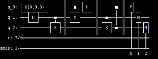
I felt a bit stuck until I learned about the deferred measurement principle. Which states that I can do the measurements later. Then, I changed a bit the algorithm to read the measurements it the end.
This means that I changed the .x(target).c_if(classic_control) to .cx(quantum_control, target) and .z(target).c_if(classic_control) to .cz(quantum_control, target).
The circuit will be something as the following. In this case $|\psi\rangle=|0\rangle$.

As for the code, it’s modified compared to the previous one. In this way, we create various quantum circuits in one shot and then send them to the quantum computer.
import matplotlib.pyplot as plt
from qiskit import *
from qiskit.tools.monitor import job_monitor
from qiskit.tools.visualization import plot_bloch_multivector, plot_histogram
from math import pi

n = 7
qcs = []
for i in range(n):
    qr = QuantumRegister(3, name="q")
    cr = ClassicalRegister(3, name="c")
    qc = QuantumCircuit(qr, cr)

    # θ = pi/2
    # θ = 0
    θ = pi*i/(n-1)
    qc.u(θ,0,0,0)

    # bell state (qubit 1: alice, qubit 2: bob)
    qc.h(1)
    qc.cx(1, 2)
    qc.barrier()

    # measurement for teleportation
    qc.cx(0,1)
    qc.h(0)
    qc.barrier()
    qc.cx(1, 2)
    qc.cz(0, 2)

    qc.measure_all()
    qcs.append(qc)

IBMQ.load_account()
provider = IBMQ.get_provider("ibm-q")
qcomp = provider.get_backend("ibm_perth")
job = execute(qcs, backend=qcomp)
real_result = job.result()
Just as an example. The result of real_result.get_counts(qcs[0]) is the following:
{'010 000': 891,
 '101 000': 96,
 '000 000': 976,
 '001 000': 872,
 '011 000': 886,
 '100 000': 75,
 '111 000': 128,
 '110 000': 76}
As we previously said, the value of interest is the most significant qubit. We want to know how many times we get 1 or 0 on that value.
This small routine will give me the results I want:
q2s = [{"0":0,"1":0} for _ in range(n)]
for i in range(n):
    tmp = real_result.get_counts(qcs[i])
    for k,v in tmp.items():
        q2s[i][k[0]]+=v
Let’s show the results in a table. What we should expect and what we really got.
| theoretical - $|0\rangle$ | theoretical - $|1\rangle$ | real - $|0\rangle$ | real - $|1\rangle$ |
|---|---|---|---|
| 1 | 0 | 0.906 | 0.094 |
| 0.933 | 0.067 | 0.857 | 0.143 |
| 0.75 | 0.25 | 0.664 | 0.336 |
| 0.5 | 0.5 | 0.492 | 0.508 |
| 0.25 | 0.75 | 0.293 | 0.707 |
| 0.067 | 0.933 | 0.162 | 0.838 |
| 0 | 1 | 0.110 | 0.890 |
As you can see, we have some reality gap. The computations in the quantum computers are going to have errors due to a number of things. One of the most important is the coherence time, which tells us that a qubit state cannot maintain its state. We have a similar table in the Qubit Rotation post, the computations are simpler and are closer to the theoretical results.
Theory (2nd part)
As I commented before, everywhere I looked for quantum teleportation I got the $|\Phi^+\rangle$ pair or $\frac{1}{\sqrt{2}} (|00\rangle + |11\rangle)$. I wanted to study a bit more and understand what happens with the other pairs. So, let’s begin again replacing equation (2) to have the following form.
$$ \begin{align} |e \rangle = \frac{1}{\sqrt{2}} (|10\rangle + |01\rangle) \end{align} $$
This is the $|\Psi^+\rangle$ according to the EPR pairs.
As before, let’s do the tensor product of $|\psi\rangle$ and the new $|e\rangle$.
$$ \begin{align*} \begin{aligned} |\psi\rangle \otimes |e\rangle &= \frac{1}{\sqrt{2}} (\alpha |0\rangle \otimes (|10\rangle + |01\rangle) + \beta |1\rangle \otimes (|10\rangle + |01\rangle))\\ &= \frac{1}{\sqrt{2}} (\alpha|010\rangle + \alpha|001\rangle + \beta|110\rangle + \beta|101\rangle) \end{aligned} \end{align*} $$
As before, we perform the following operations to transport the information.
$$ \begin{align*} \begin{aligned} &(H \otimes I \otimes I) (CNOT \otimes I) (|\psi\rangle \otimes |e\rangle)\\ &=(H \otimes I \otimes I) (CNOT \otimes I) \frac{1}{\sqrt{2}} (\alpha|010\rangle + \alpha|001\rangle + \beta|110\rangle + \beta|101\rangle) \\ &= (H \otimes I \otimes I) \frac{1}{\sqrt{2}} (\alpha|010\rangle + \alpha|001\rangle + \beta|100\rangle + \beta|111\rangle) \\ &= \frac{1}{2} (\alpha(|010\rangle + |110\rangle + |001\rangle + |101\rangle) + \beta(|000\rangle + |011\rangle - |100\rangle - |111\rangle)) \\ \end{aligned} \end{align*} $$
$$ \begin{align*} \begin{aligned} = \frac{1}{2}( & \phantom{+} |00\rangle (\alpha|1\rangle + \beta|0\rangle) \hphantom{\quad )} \\ & + |01\rangle (\alpha|0\rangle + \beta|1\rangle) \hphantom{\quad )}\\ & + |10\rangle (\alpha|1\rangle - \beta|0\rangle) \hphantom{\quad )}\\ & + |11\rangle (\alpha|0\rangle - \beta|1\rangle) \quad )\\ \end{aligned} \end{align*} $$
As in the previous section on theory, we can create a table with the needed operations to obtain $|\psi\rangle$.
| $|q_0q_1\rangle$ | $|q_2\rangle$ state | Quantum Gate |
|---|---|---|
| $|00\rangle$ | $\alpha|1\rangle + \beta|0\rangle$ | $X$ |
| $|01\rangle$ | $\alpha|0\rangle + \beta|1\rangle$ | $I$ |
| $|10\rangle$ | $\alpha|1\rangle - \beta|0\rangle$ | $ZX$ |
| $|11\rangle$ | $\alpha|0\rangle - \beta|1\rangle$ | $Z$ |
Anyway, with this information we are ready to meet practice.
Practice (2nd Part)
We won’t even bother to try c_if because we know it does not work in the quantum computer. You’ll find in the code two comments which refer to line to get the new entangled state as well as a transformation (X gate) we have to perform to be able to use the controlled X gate (if we analyze the previous table, we realize that we need to flip the bit to control the X in a deferred configuration).
import matplotlib.pyplot as plt
from qiskit import *
from qiskit.tools.monitor import job_monitor
from qiskit.tools.visualization import plot_bloch_multivector, plot_histogram
from math import pi

n = 7
qcs = []
for i in range(n):
    qr = QuantumRegister(3, name="q")
    qc = QuantumCircuit(qr)

    θ = pi*i/(n-1)
    qc.u(θ,0,0,0)

    # bell state
    qc.h(1)
    qc.cx(1, 2)
    # NEW next line to have the |01>+|10> state
    qc.x(1)
    qc.barrier()

    # measurement for teleportation
    qc.cx(0,1)
    qc.h(0)
    qc.barrier()
    # NEW nex line to control as needed
    qc.x(1)
    qc.cx(1, 2)
    qc.cz(0, 2)

    qc.measure_all()
    qcs.append(qc)

IBMQ.load_account()
provider = IBMQ.get_provider("ibm-q")
qcomp = provider.get_backend("ibm_perth")
job = execute(qcs, backend=qcomp)
real_result = job.result()
Each one of the circuits are similar as the following.

Now, I leave you the results in the following table.
| theoretical - $|0\rangle$ | theoretical - $|1\rangle$ | real - $|0\rangle$ | real - $|1\rangle$ |
|---|---|---|---|
| 1 | 0 | 0.900 | 0.100 |
| 0.933 | 0.067 | 0.854 | 0.146 |
| 0.75 | 0.25 | 0.679 | 0.321 |
| 0.5 | 0.5 | 0.508 | 0.492 |
| 0.25 | 0.75 | 0.294 | 0.706 |
| 0.067 | 0.933 | 0.142 | 0.858 |
| 0 | 1 | 0.116 | 0.884 |
Concerning the numerical values, there is nothing more to be said that the conclusion in the first practical part. However, we can see that we can perform a quantum teleportation with another type of pair. I did a small computation for every one of the pairs in the my written notes, I was mainly thinking in terms of triplets and singlet states.
