Quantum Computation Qubit Rotation
This summer break I had some time to read Quantum Mechanics: The Theoretical Minimum. Now I kind of want to make some test about some of the lectures.
Theory
This article concerns the first test I wanted to do and is based on the third lecture. This is where the pauli matrices ($\sigma_x$, $\sigma_y$ and $\sigma_z$) are introduced as well as the composition of a general matrix $\sigma_n$. This can be viewed as follows.
$$ \begin{align*} \begin{split} \sigma_n & = \vec{n} \cdot \vec{\sigma} \\ & = n_x \sigma_x + n_y\sigma_y+n_z\sigma_z \\ & =n_x\begin{pmatrix} 0 & 1 \\ 1 & 0 \end{pmatrix}+n_y\begin{pmatrix} 0 & i \\ -i & 0 \end{pmatrix} + n_x\begin{pmatrix} 1 & 0 \\ 0 & -1 \end{pmatrix} \\ & =\begin{pmatrix} n_z & n_x-in_y \\ n_x+in_y & -n_z \end{pmatrix} \end{split} \end{align*} $$
The last is the Equation (3.23) in the book.
Thus, section 3.7 implements equation (3.23) with the following values $$ \begin{align*} \begin{split} n_z = \cos \theta \\ n_x = \sin \theta \\ n_y = 0 \end{split} \end{align*} $$
Plugging in we have, $$ \begin{equation} \sigma_n = \begin{pmatrix} \cos \theta & \sin \theta \\ \sin \theta & -\cos \theta \end{pmatrix} \end{equation} $$
With the following eigenvalues and eigenvectors:
$$ \lambda_1 = 1 \qquad |\lambda_1 \rangle = \begin{pmatrix} \cos \frac{\theta}{2} \\ \sin \frac{\theta}{2} \end{pmatrix} $$ $$ \lambda_2 = -1 \qquad |\lambda_1 \rangle = \begin{pmatrix} -\sin \frac{\theta}{2} \\ \cos \frac{\theta}{2} \end{pmatrix} $$
Now, for the important part, we want to know the probability of observing $\sigma_n=+1$ and $\sigma_n=-1$.
$$ P(+1) = \langle 0 | \lambda_1 \rangle \langle \lambda_1 | 0 \rangle = \cos^2 \frac{\theta}{2} $$
$$ P(-1) = \langle 0 | \lambda_2 \rangle \langle \lambda_2 | 0 \rangle = \sin^2 \frac{\theta}{2} $$
Practice
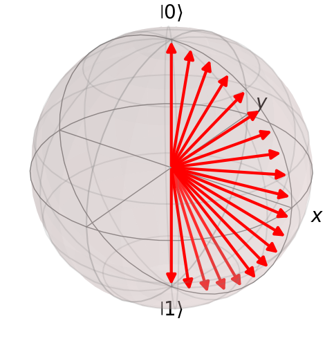
Let’s say I have several states which are created based on equation (1). If we plot several values of $\theta$ we can have a representation in the bloch sphere as in the following picture.

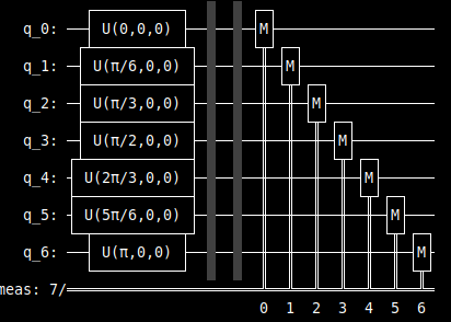
What we want to know is if the theory gives the value of reality. Thus we implement a quantum circuit. We are going to use only 7 states to see what the results are. The 7 states are because we are going to use a quantum computer with 7 qubits (that’s what we have in the IBM quantum experience).
from math import pi
import matplotlib.pyplot as plt
from qiskit import *
from qiskit.tools.visualization import plot_bloch_multivector, plot_histogram
from qiskit.quantum_info import state_fidelity
from qiskit import BasicAer
import numpy as np
n = 7
qc = QuantumCircuit(n)

th_res = []  # theoretical results
for i in range(n):
    θ = pi*i/(n-1)
    qc.u(θ, 0, 0, i)
    # compute theoretical results
    tmp = {"0": np.cos(θ/2)**2, "1": np.sin(θ/2)**2}
    th_res.append(tmp)

qc.barrier()
qc.measure_all()

qc.draw()

backend = BasicAer.get_backend('qasm_simulator')
# uncomment next 2 lines to use a quantum computer from IBM
# provider = IBMQ.get_provider("ibm-q")
# backend = provider.get_backend("ibm_perth")
shots = 1024
results = execute(qc, backend=backend, shots=shots).result()
answer = results.get_counts()

res = [{"0": 0, "1": 0} for _ in range(n)]
for i in range(n):
    for k, v in answer.items():
        res[i][k[i]] += v
    res[i]["0"] /= shots
    res[i]["1"] /= shots

df_th = pd.DataFrame(th_res)
df_res = pd.DataFrame(res[::-1]) # reversed order
The drawn circuit is as follows:

As for the results, you can see the theoretical (theo), simulated (sim) and real (real) results from the ibm_perth quantum computer from IBM.
| theo - $|0\rangle$ | theo - $|1\rangle$ | sim - $|0\rangle$ | sim - $|1\rangle$ | real - $|0\rangle$ | real - $|1\rangle$ |
|---|---|---|---|---|---|
| 1 | 0 | 1 | 0 | 0.973 | 0.027 |
| 0.933 | 0.067 | 0.935 | 0.065 | 0.891 | 0.109 |
| 0.75 | 0.25 | 0.763 | 0.237 | 0.632 | 0.368 |
| 0.5 | 0.5 | 0.528 | 0.472 | 0.478 | 0.522 |
| 0.25 | 0.75 | 0.25 | 0.75 | 0.283 | 0.717 |
| 0.067 | 0.933 | 0.073 | 0.927 | 0.1 | 0.9 |
| 0 | 1 | 0 | 1 | 0.019 | 0.981 |
You can notice the results seem to fit reality. What might bother people is mainly the extremes in the real columns, but we have several quantum effects which give us some errors (this of course doesn’t happen in simulation though). In the end, these errors are natural in the current state of the art quantum computers.
You can find the code in the following gist. Where you will find the code for plotting the bloch sphere that is in the article as well.
To me, it was a nice experience. I have played with quantum circuits before, but not necessarily thinking about the fundamental theory.
