Exploiting Structure Linear Algebra Solver
Intro
Today I wanted to talk about one of the most basic equations that we can use in linear algebra.
$$ Ax=b $$
This is one of those ubiquitous formulas that you can’t escape. You have various applications in economics, robotics, computer vision, optimization, chemistry and a lot more topics.
Sometimes however, you can encounter really big problems which are going to be really slow to solve or sometimes you really need a low latency system, in any of those cases, you need to know a little bit more, how you can efficiently solve pour problem.
FLOPS
(FL)oating point (OP)erations is the measurement usually used. Let’s give some examples.
- Scalar Vector Multiplication: $ax$ where $a \in \mathbb{R}$ and $x \in \mathbb{R}^n$ ($a$ is a float and $x$ is a vector of floats of length $n$) will take $n$ flops, this equation is linear. In $\mathcal{O}$ notation $\mathcal{O}(n)$.
- Inner Product: $\langle x, y \rangle$ where $x,y \in \mathbb{R}^n$ will take $n$ multiplications and $n-1$ summations, thus $2n-1$ flops (also $\mathcal{O}(n)$).
- Matrix Vector Product: $Ax$ where $A \in \mathbb{R}^{n,m}$ and $x \in \mathbb{R}^m$ corresponds to taking the inner product for the $n$ rows, giving $n(2m-1)=2nm-m$flops. This is quadratic, because $\mathcal{O}(nm)$ if we take a squared matrix (i.e. $n=m$) then $\mathcal{O}(n^2)$.
For more you can see more number of flops per operation in this reference.
FLOPS on Linear Equations
In the case of solving $Ax=b$ for $x$, the solution takes the order of $\mathcal{O}(n^3)$. This is something good to take into account, because you can see as your problem grows, the number of computations grows on the third order, which can be very costly. However, there are some cases in which $Ax=b$ can be computed faster.
- Diagonal Matrix: $x=A^{-1}b=(b_1/a_{11}, \dots, b_n/a_{nn})$ takes only $n$ flops.
- Lower Triangular and Upper Triangular Matrices: $\mathcal{O}(n^2)$
- Orthogonal Matrices: $\mathcal{O}(n^2)$ for a general case (faster in the case $A=I-2uu^\mathsf{T}$ which is around $4n$ flops)
- Permutation Matrix this particular case is $0$ flops because $A=A^{-1}=A^\mathsf{T}$.
More information in this pdf extracted from a convex optimization course (and which is actually the motivation for this post).
Configuration
In this article, I consider the reader to have some language of the julia programming language.
First we load some packages.
using SparseArrays
using LinearAlgebra
using BandedMatrices
using SpecialMatrices
using ToeplitzMatrices
using Random
using BlockArrays
using FFTW
To have a reference. The computer where I’m testing has the processor Intel Core i7-10510U @ 8x 4.9GHz and 16Gb RAM.
Diagonal Matrix
Well, we already said that a diagonal matrix should take $\mathcal{O}(n)$ flops. We can now compare it in different ways.
n = 5000;
y = rand(n);

# Diagonal Matrix
a = rand(n);  # vector
A = diagm(a); # diagonal dense
A_d = Diagonal(a); # diagonal type
Asp = spdiagm(a);  # sparse type
x = A\y;
x = A_d\y;
x = Asp\y;
x = y./a;
The four last lines will create the same result. In order to compare them, let’s benchmark them.
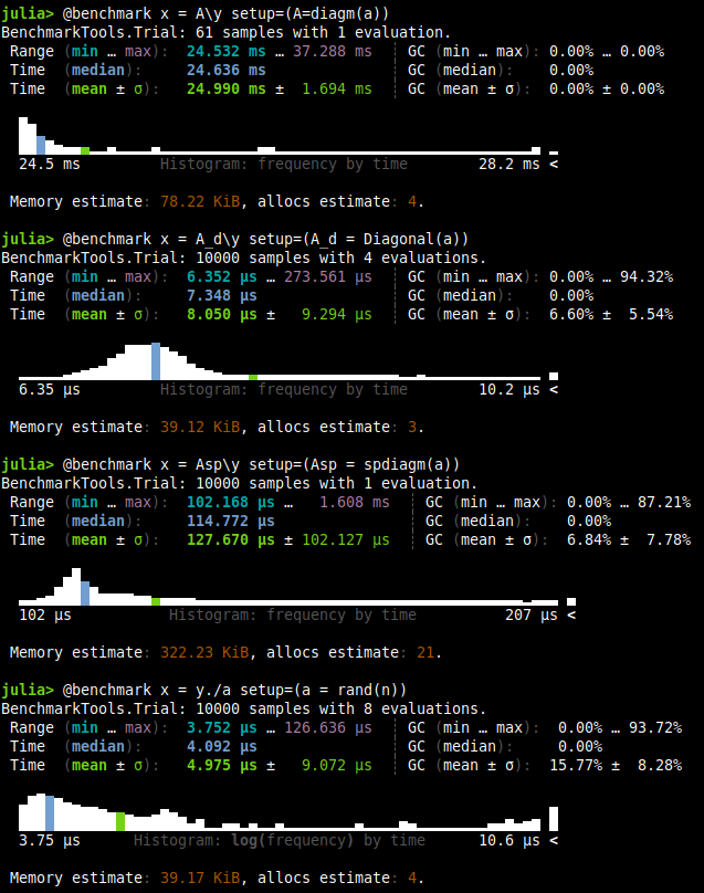
You can see that only 61 samples where generated for the dense matrix. If we take only the mean of each benchmark, we end up with the following table.
| Test | Time |
|---|---|
| Dense | 24.99 ms |
| Diagonal | 8.05 μs |
| Sparse | 127.67 μs |
| Vector | 4.9 μs |
Of course the winner is the vector, because there is no overhead in the type nor function overloading or anything else. However, the times are crazy, from vector to sparse we have 25x times, and well vector compared to dense is around 5000x slower.
Notice the memory usage in each one of the benchmarking. It’s not only faster but lighter in consumption . This will be true for all the following sections too.
Banded Matrix
Is a sparse matrix whose non-zero entries are confined to a diagonal band. Such as the following:
$$ \begin{bmatrix} B_{11} & B_{12} & 0 & \cdots & \cdots & 0 \\ B_{21} & B_{22} & B_{23} & \ddots & \ddots & \vdots \\ 0 & B_{32} & B_{33} & B_{34} & \ddots & \vdots \\ \vdots & \ddots & B_{43} & B_{44} & B_{45} & 0 \\ \vdots & \ddots & \ddots & B_{54} & B_{55} & B_{56} \\ 0 & \cdots & \cdots & 0 & B_{65} & B_{66} \end{bmatrix} $$
Here is the wikipedia definition.
So, in julia there is the type BandedMatrix that we test in this subsection.
Abd = BandedMatrix(-1=> rand(n-1), 0=> rand(n), 1=>rand(n-1));
Asp = spdiagm(-1=> rand(n-1), 0=> rand(n), 1=>rand(n-1));
A = Array(Abd);
x = A\y; # dense
x = Abd\y; # banded
x = Asp\y; # sparse
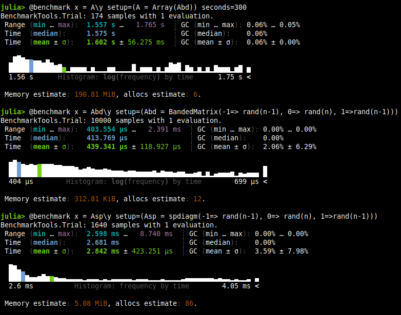
| Test | Time |
|---|---|
| Dense | 1.6 s |
| Banded | 439.34 μs |
| Sparse | 2.842 ms |
I believe that there is nothing more to be said when we see the numbers. According to this course in convex optimization, If $A$ is $k$-banded, it costs about $nk^2$ flops which explains pretty well our behavior.
Circulant Matrix
This is one of those cases where the sparse matrix is not useful because we actually have a dense matrix, the structure comes by repetition of terms (see wiki) as follows:
$$ C={\begin{bmatrix}c_{0}&c_{n-1}&\cdots &c_{2}&c_{1}\\c_{1}&c_{0}&c_{n-1}&&c_{2}\\\vdots &c_{1}&c_{0}&\ddots &\vdots \\c_{n-2}&&\ddots &\ddots &c_{n-1}\\c_{n-1}&c_{n-2}&\cdots &c_{1}&c_{0}\\\end{bmatrix}} $$
Without further ado, let’s go to the code and benchmark.
Acr = Circulant(rand(n));
A = Array(Acr);
x = A\y; # dense
x = Acr\y; # circulant
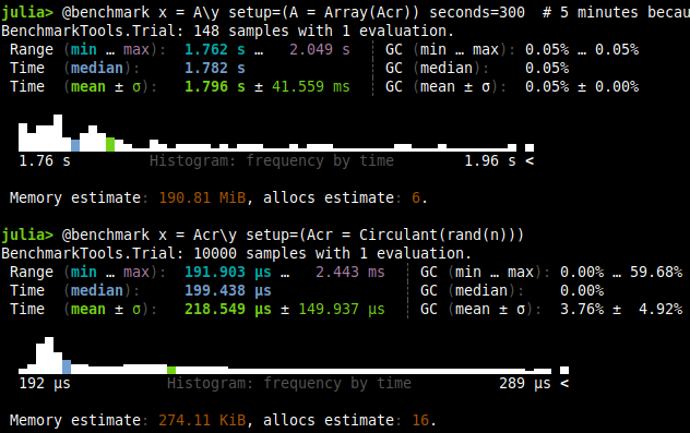
| Test | Time |
|---|---|
| Dense | 1.8 s |
| Circulant | 218.54 μs |
Again, this takes around 1000x more time for a $n=5000$.
Other matrices
In julia, you can find the package SpecialMatrices.jl where you can find Hilbert, Kahan, Vanderdmonte and more kind of matrices.
Elephant in the room (LU decomposition)
So, this guy forgot about LU decomposition. Well, one of the first that you will learn, it’s that when possible, we can convert the matrix
$$ LU=PA $$
Where $L$ is a lower triangular matrix, $U$ is an upper triangular matrix and $P$ is a permutation matrix. This will allow us to have a system of matrices that will solve our linear system.
n = 1000;
y = rand(n);
A = rand(n,n);
luA=lu(A);
@benchmark x=A\y setup=(A=rand(n,n))
@benchmark lu(A) setup=(A=rand(n,n))
@benchmark luA\y setup=(luA=lu(A))
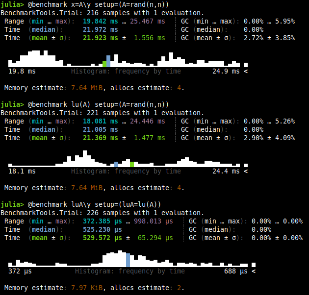
As you can see, the first two benchmark are pretty close one to another. Thus, the LU decomposition takes almost as much time as the solving (perharps because the solver does something similar first, it actually depends on the case). The LU solution however, we can store it to use it later. As you can see in the third benchmark, the computation is really fast, $\mathcal{O}(n^2)$ according to this post. While the normal solver for a dense matrix takes $\mathcal{O}(n^3)$ as we stated before.
You can see a bit more in this link which will also tackle sparse LU decomposition.
Matrix with Extended Structure
Let’s say now you have the following block matrix.
$$ \begin{bmatrix}A&B\\C&D\end{bmatrix}\begin{bmatrix}x_1\\x_2\end{bmatrix}=\begin{bmatrix}y_1\\y_2\end{bmatrix} $$
Imagine now that the $A$ variable is a big diagonal matrix compared to the rest of the matrix as the following picture.

This kind of pattern is crying to be solved in an efficient manner. So how do we exploit structure? I was actually a bit stock and I asked Math StackExchange for some help. I got the help in the comment section hinting to the Schur Complement.
$$ \begin{split} x_1=A^{-1}(y_1-Bx_2)\\ \left(D-CA^{-1}B\right)x_2=y_2-CA^{-1}y_1 \end{split} $$
Notice that we need $A$ to be non-singular (invertible) for this to work.
So, let’s solve our system.
n = 5000;
n_ext = Int(round(n*1.01));
y_1 = rand(n);
y_2 = rand(n_ext-n);
y = mortar([y_1,y_2]);
a = rand(n);

A = Diagonal(a);
B = rand(n, n_ext-n);
C = rand(n_ext-n,n);
D = rand(n_ext-n,n_ext-n);

AA = Array(mortar(reshape([A,C,B,D],2,2)));
y = Array(y);

AA_sp = sparse(AA);


x = AA\y; # dense
x = AA_sp\y; # sparse

# solving with structure
tmp1 = y_2-C*(A\y_1);
tmp2 = D-C*(A\B);
x_2 = tmp2\tmp1;
x_1 = A\(y_1-B*x_2);
x = mortar([x_1,x_2]);
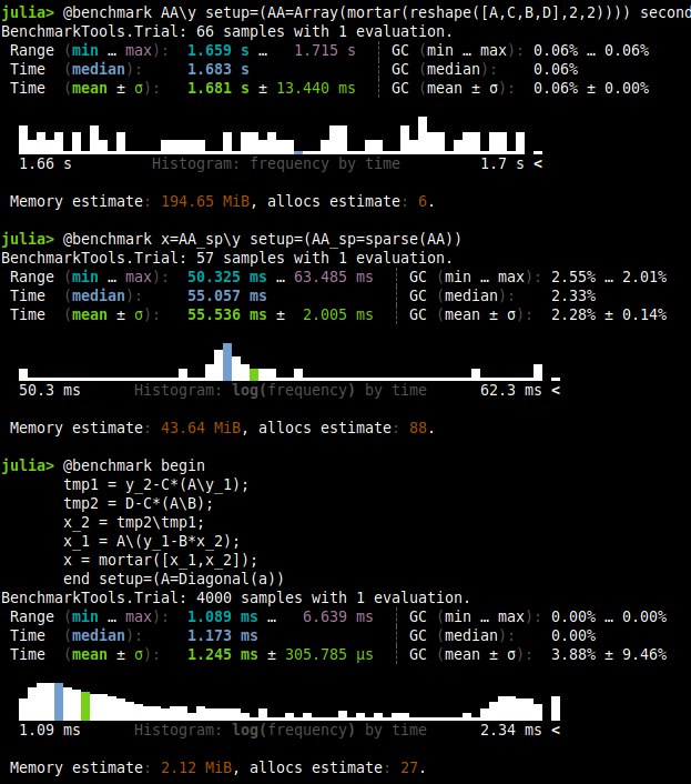
| Test | Time |
|---|---|
| Dense | 1.68 s |
| Sparse | 55.53 ms |
| Structure Exploited | 1.245 ms |
Remember, this is a $5050\times 5050$ matrix with a $5000\times 5000$ diagonal matrix in block $A$. Thus, by exploiting structure, we have >1000x times better performance than the dense and around 50x faster than the sparse counterpart. I believe this is a huge deal. Look also at the memory usage, it’s way better for the one where we exploited structure.
Additionally, this kind of problem can have instead of a diagonal matrix, a circular matrix or some other type. This will allow us some speed up where sparsity is incapable.
Structured matrix plus low rank term
Another case extracted from this convex optimization course is when you have an structured matrix plus a low rank, as the following:
$$ (A+BC)x=b $$
Developing the equation a bit, we can show that it’s the same as.
$$ \begin{bmatrix}A&B\\C&-I\end{bmatrix}\begin{bmatrix}x\\y\end{bmatrix}= \begin{bmatrix}b\\0\end{bmatrix} $$
Which by Schur Complement (our previous example), we know how to solve.
As a side note, this reminds me of the Woodbury Identity.
References
You can find the reference gist I created for this post. Inside the post, you’ll also find more references.
