On Ellipsis from sincos and numerical range

In the past couple of days I stumbled into an interesting problem (Problem 35) in the book Problems and Solutions in Introductory and Advanced Matrix Calculus by W. Steeb.

So, during the process of deciphering one section, I starting plotting to visualize a bit better and I stumbled into the following picture.

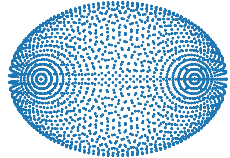
It captivated me and I decided to write an entry about it.

The problem

The problem asks to find the numerical range of some matrices. Defining the numerical range as: $$ \begin{equation} F(A)=\{z^*Az \vert \|z\|=1,z \in \mathbb{C}^n\} \end{equation} $$

From Toeplitz-Hausdorff convexity theorem, the numerical range of a square matrix is a convex compact subset of the complex plane, see more here.

In the definition of the problem, the following matrix $C$ is used.

$$ C= \begin{pmatrix} 0&0 \\ 1 & 1 \end{pmatrix} $$

In order to have $\Vert z \Vert=1$ in the 2 dimensional case we need the values of $z$ to be as follows. $$ z= \begin{pmatrix} e^{i\phi} \cos \theta \\ e^{i\chi }\sin\theta \end{pmatrix}\qquad \phi,\chi,\theta \in \mathbb{R} $$ To see why this is the case, you can see it visually in the real plane in the first image of this section. Or algebraically:

$$ \begin{split} z^*z&=e^{i\phi-i\phi}\cos^2 \theta+e^{i\chi-i\chi}\sin^2 \theta \\ &=e^{0}\cos^2 \theta+e^{0}\sin^2 \theta \\ &=\cos^2 \theta+\sin^2 \theta \\ &=1 \end{split} $$

Then, when we solve for $F(C)$ we get. $$ F(C)=z^*Cz=e^{i(\phi-\chi)}\sin\theta\cos\theta +\sin^2\theta $$ Without loss of generality $p=\phi-\chi \in \mathbb{R}$, thus: $$ \begin{equation} z^*Cz=e^{ip}\sin\theta\cos\theta +\sin^2\theta \end{equation} $$

Given that $e^{ip}$ represents a rotation in the complex plane, the values of $p \in [0,2\pi]$. Also, as $\sin$ and $\cos$ are trigonometric functions, the values are $\theta \in [0,2\pi]$.

In the solution material, something that stroke me was this last remark.

Thus, the numerical range $F(C)$ is the closed elliptical disk in the complex plane with foci at $(0,0)$ and $(1,0)$, minor axis $1$ and major axis $\sqrt{2}$

I did not understand why. So I decided that I needed to graph what it was going on.

Code

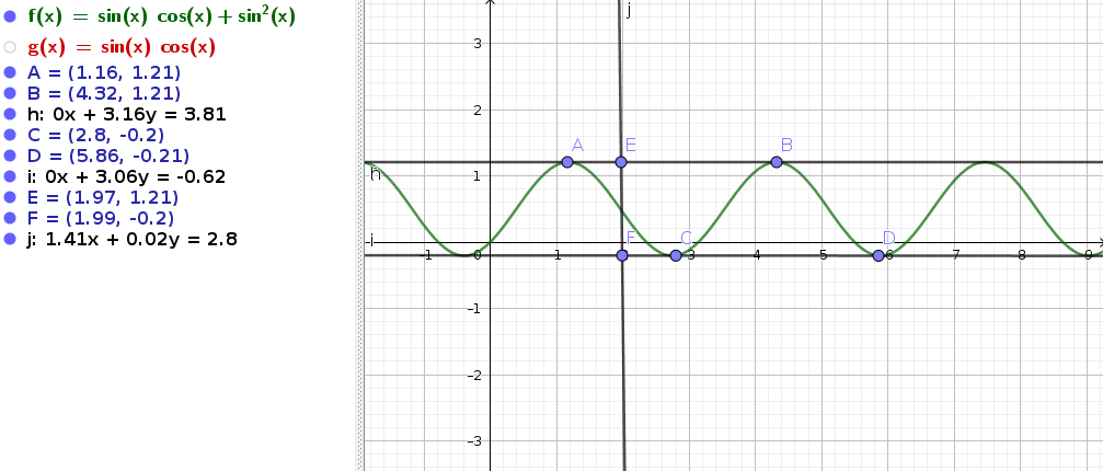
The first try was to do something in geogebra (I was actually in bed and that’s the only thing I have in my reader to plot). You can see the result in the following image. The geogebra code is here.

import numpy as np
import matplotlib.pyplot as plt
p = np.linspace(0,1j*2*np.pi,50) # p is ip
θ = np.linspace(0,np.pi/2,50)
P,Θ = np.meshgrid(p,θ)
m = np.exp(P)*np.sin(Θ)*np.cos(Θ) + np.sin(Θ)**2
b = m.flatten()
r,i = np.real(b), np.imag(b)
plt.scatter(r,i)
plt.axis('equal')
plt.show()

Which gives the following image.

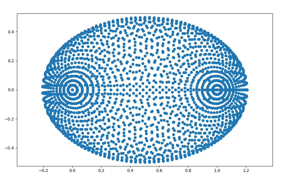
This image suggests strongly the values given by the quotation.

Thus, the numerical range $F(C)$ is the closed elliptical disk in the complex plane with foci at $(0,0)$ and $(1,0)$, minor axis $1$ and major axis $\sqrt{2}$

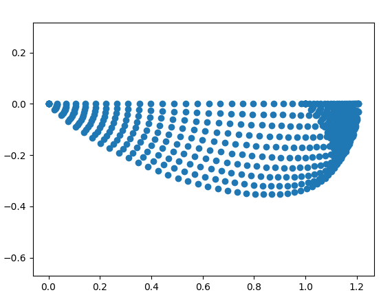
However, this beautiful pattern is a feature of our sampling $\theta$. You can see it with the following two pictures.

With p = np.linspace(7/8*1j*2*np.pi,1j*2*np.pi,10)

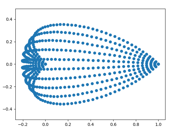
More

At this point, I was somehow reminded kind of analogous convex optimization problems. Fitting Hyper Spheres and Hyper Ellipsoids strongly came into my mind, because of course the ellipsoids (ellipses in 2D) are represented in matrices. The Convex Optimization Book in Section 2.2.2 defines the ellipsoid as the following: $$ \begin{equation} \mathcal{E}=\left\{ x_c + Au \, | \, \|u\|_2 \leq 1 \right\} \end{equation} $$ We can see strong similarities with equation (1).

I was also thinking that the eigenvalues and eigenvectors should have something to do, since for a semidefinite matrix. $$ C-\lambda I=0 $$ This gives $$ \lambda (\lambda-1) $$ Thus $\lambda_1=0$ and $\lambda_2=1$. These are suspiciously the same values as the focus points. However well, the eigenvectors didn’t tell me that much. $$ v_1 = \begin{pmatrix} 1 \\ 0 \end{pmatrix}\quad v_2 = \begin{pmatrix} 1 \\ -1 \end{pmatrix} $$

Then, I stumbled into The numerical range ellipse, where they compute the minor axis and major axis.

$$ b^2 = \operatorname{tr}(A^*A) − |\lambda_1|^2 − |\lambda_2|^2. $$

This is actually Theorem 6.1 of Finding Ellipsis

import numpy as np
A = np.array([[0,0],[1,1]])
λs = np.linalg.eigvals(A)
minor = np.sqrt(np.trace(np.conj(A.T)@A)-(λs**2).sum())

The value of minor is 1 as the book. In any case, I still have a bit of work to find the major axis, add more examples and something extra. I will add them in the following days (if I don’t forget).

References

• [Book] Finding Ellipses: What Blaschke Products, Poncelet’s Theorem, and the Numerical Range Know about Each Other (see link).
• Presentation by Tin-Yau Tam
• John D. Cook blog entry
• gist