Chebyshev Polynomials Fitting

The Chebyshev polynomials are two sequences of polynomials related to the cosine and sine functions. $$ \begin{align*} \begin{split} {\displaystyle T_{n}(\cos \theta )=\cos(n\theta )}\\ {\displaystyle U_{n}(\cos \theta )\sin \theta =\sin {\big (}(n+1)\theta {\big )}} \end{split} \end{align*} $$

One of the interesting properties of this kind of polynomials is that the dot product of a series $T_n$ (or $U_n$) with respect to another $T_m$ (or $U_m$) is orthogonal when $n \neq m$.

$$ \int_{-1}^{1}T_n (x)\,T_{m}(x)\,{\frac{\mathrm{d} x}{\sqrt {1-x^{2}}}}={ \begin{cases}0&~{\text{ if }}~n\neq m,\\ \pi &~{\text{ if }}~n=m=0,\\ {\frac {\pi }{2}}&~{\text{ if }}~n=m\neq 0.\end{cases}} $$

Orthogonality allow us to store less information, because the information is non redundant. Furthermore, we can see from the definition that we have the functions $\sin$ and $\cos$. Therefore, the stable interval will be $[-1,1]$ (This is also true in numerical functions such as chebval).

Thus a $T$ type chebyshev polynomial can be seen as follows:

$$ \begin{equation} p(x) = c_0 + c_1 T_1(x) + … + c_n T_n(x) \end{equation} $$

Example

This example is going to be partially code and partially equations. So let’s start some initialization parameters that we are going to use later.

import numpy as np
from numpy.polynomial import chebyshev as C
import matplotlib.pyplot as plt
from  scipy.special import eval_chebyt
import cvxpy as cp

Now, let’s have the following function as a random sampler:

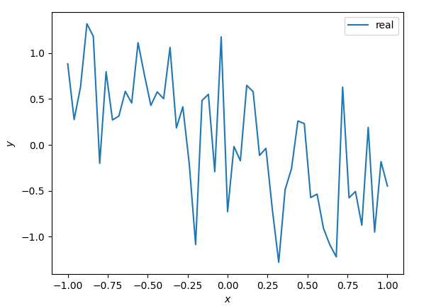
$$ \begin{equation} y = x^3-x+\varepsilon \end{equation} $$ where $\varepsilon \in \mathcal{N}(0,.5)$ and the interval of the function is $[-1,1]$. The function is shown in the following code and picture.

np.random.seed(0)
n = 51
x = np.linspace(-1, 1, n)
y = x**3 - x + .5*np.random.randn(n)
plt.xlabel("$x$")
plt.ylabel("$y$")
plt.plot(x, y, label="real")
plt.legend()

We actually won’t care about (2) anymore, it was just useful to generate some points near the specified interval.

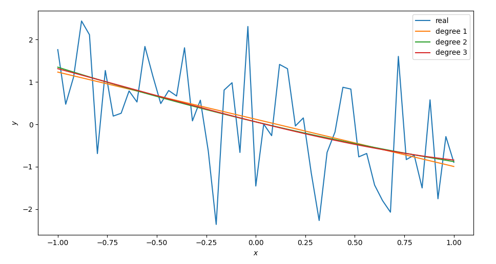
Let’s fit some fitting with polynomials of degree 1,2 and 3.

plt.plot(x, y, label="real")
for degree in range(1, 4):
    c, _ = C.chebfit(x, y, degree, full=True)
    y_pred = C.chebval(x, c)
    plt.plot(x, y_pred, label=f"degree {degree}")
plt.legend()
plt.xlabel("$x$")
plt.ylabel("$y$")

Well, that was kind of easy. We fit the chebyshev $T$ with various degrees and we saw that for this particular function, the polynomials are not so far apart, thus, the polynomial of order 1 seems to do the work.

More fitting

When I was digging into this I felt like something was missing. Because I didn’t understand how this fitting was done. Thus, we have the following fit.

n_degree = 4
c, stats = C.chebfit(x, y, n_degree, full=True)
# c = array([ 0.16322587, -1.10155228,  0.12751551,  0.02381081,  0.08877683])

The c variable is the vector $c=(c_0,c_1, \dots, c_n)$ referred in (1). Thus, if we are going to hand-make a fitting function. Now, let’s create a matrix $A$ that maps all the values of x in the chebyshev function.

$$ \begin{split} A &= \begin{bmatrix} | & | & | & | \\ T_0 & T_1 & \dots & T_n \ \\ | & | & | & | \\ \end{bmatrix} \\ &= \begin{bmatrix} T_0(x_0) & T_1(x_0) & \dots & T_n(x_0) \ \\ T_0(x_1) & T_1(x_1) & \dots & T_n(x_1) \ \\ \vdots & \vdots & \vdots & \vdots \\ T_0(x_m) & T_1(x_m) & \dots & T_n(x_m) \ \\ \end{bmatrix} \end{split} $$

A = np.c_[[eval_chebyt(n_, x) for n_ in range(n_degree+1)]].T

As you can see, the function eval_chebyt corresponds to $T_n$. Once we have this problem, we can solve for the Linear Least Squares.

$$ \| A\hat{x}-y\|^2_2 $$

c_ = np.linalg.lstsq(A, y)
# c_[0] = array([ 0.16322587, -1.10155228,  0.12751551,  0.02381081,  0.08877683])

As we can see, the values of c and c_[0] are the same.

This problem is convex. Thus, we could use cvxpy to solve the problem and if needed, add further constraints for more specific problems. I leave the example without constraints:

x_cvx = cp.Variable(n_degree+1)
cost = cp.sum_squares(A @ x_cvx - y)
prob = cp.Problem(cp.Minimize(cost))
prob.solve()
# x_cvx.value = array([ 0.16322587, -1.10155228,  0.12751551,  0.02381081,  0.08877683]

References

This work is based on a Gist I created some months ago.